DataScience/TensorFlow[ANN]
딥러닝 텐서플로우 이미지 10개로 분류 Saving architecture & Saving network weights, Dropout, validation_data, Flatten안쓰기
leopard4
2022. 12. 29. 15:05
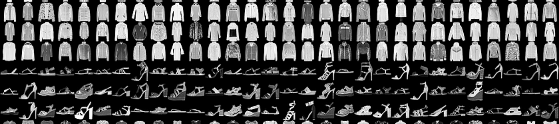 Image source: https://www.kaggle.com/
Stage 1: Installing dependencies
In [1]:
# 코랩은 이미 깔려잇어 pass
In [1]:
Stage 2: Import dependencies for the project
In [2]:
import numpy as np
import tensorflow as tf
from tensorflow.keras.datasets import fashion_mnist
Stage 3: Dataset preprocessing
Loading the dataset
In [3]:
(X_train,y_train),(X_test,y_test)= fashion_mnist.load_data() # 넘파이로 받아옴 // (X_train,y_train),(X_test,_y_test) 텐서플로우 규칙.
Downloading data from https://storage.googleapis.com/tensorflow/tf-keras-datasets/train-labels-idx1-ubyte.gz
29515/29515 [==============================] - 0s 0us/step
Downloading data from https://storage.googleapis.com/tensorflow/tf-keras-datasets/train-images-idx3-ubyte.gz
26421880/26421880 [==============================] - 0s 0us/step
Downloading data from https://storage.googleapis.com/tensorflow/tf-keras-datasets/t10k-labels-idx1-ubyte.gz
5148/5148 [==============================] - 0s 0us/step
Downloading data from https://storage.googleapis.com/tensorflow/tf-keras-datasets/t10k-images-idx3-ubyte.gz
4422102/4422102 [==============================] - 0s 0us/step
In [4]:
X_train.shape
Out[4]:
(60000, 28, 28)
In [5]:
X_test.shape
Out[5]:
(10000, 28, 28)
Image normalization
In [6]:
X_train[0] # 리스트의 액세스 첫번째 이미지 가져오기 // 또한 X_train[ , , ] 가능 (넘파이억세스)
Out[6]:
array([[  0,   0,   0,   0,   0,   0,   0,   0,   0,   0,   0,   0,   0,
          0,   0,   0,   0,   0,   0,   0,   0,   0,   0,   0,   0,   0,
          0,   0],
       [  0,   0,   0,   0,   0,   0,   0,   0,   0,   0,   0,   0,   0,
          0,   0,   0,   0,   0,   0,   0,   0,   0,   0,   0,   0,   0,
          0,   0],
       [  0,   0,   0,   0,   0,   0,   0,   0,   0,   0,   0,   0,   0,
          0,   0,   0,   0,   0,   0,   0,   0,   0,   0,   0,   0,   0,
          0,   0],
       [  0,   0,   0,   0,   0,   0,   0,   0,   0,   0,   0,   0,   1,
          0,   0,  13,  73,   0,   0,   1,   4,   0,   0,   0,   0,   1,
          1,   0],
       [  0,   0,   0,   0,   0,   0,   0,   0,   0,   0,   0,   0,   3,
          0,  36, 136, 127,  62,  54,   0,   0,   0,   1,   3,   4,   0,
          0,   3],
       [  0,   0,   0,   0,   0,   0,   0,   0,   0,   0,   0,   0,   6,
          0, 102, 204, 176, 134, 144, 123,  23,   0,   0,   0,   0,  12,
         10,   0],
       [  0,   0,   0,   0,   0,   0,   0,   0,   0,   0,   0,   0,   0,
          0, 155, 236, 207, 178, 107, 156, 161, 109,  64,  23,  77, 130,
         72,  15],
       [  0,   0,   0,   0,   0,   0,   0,   0,   0,   0,   0,   1,   0,
         69, 207, 223, 218, 216, 216, 163, 127, 121, 122, 146, 141,  88,
        172,  66],
       [  0,   0,   0,   0,   0,   0,   0,   0,   0,   1,   1,   1,   0,
        200, 232, 232, 233, 229, 223, 223, 215, 213, 164, 127, 123, 196,
        229,   0],
       [  0,   0,   0,   0,   0,   0,   0,   0,   0,   0,   0,   0,   0,
        183, 225, 216, 223, 228, 235, 227, 224, 222, 224, 221, 223, 245,
        173,   0],
       [  0,   0,   0,   0,   0,   0,   0,   0,   0,   0,   0,   0,   0,
        193, 228, 218, 213, 198, 180, 212, 210, 211, 213, 223, 220, 243,
        202,   0],
       [  0,   0,   0,   0,   0,   0,   0,   0,   0,   1,   3,   0,  12,
        219, 220, 212, 218, 192, 169, 227, 208, 218, 224, 212, 226, 197,
        209,  52],
       [  0,   0,   0,   0,   0,   0,   0,   0,   0,   0,   6,   0,  99,
        244, 222, 220, 218, 203, 198, 221, 215, 213, 222, 220, 245, 119,
        167,  56],
       [  0,   0,   0,   0,   0,   0,   0,   0,   0,   4,   0,   0,  55,
        236, 228, 230, 228, 240, 232, 213, 218, 223, 234, 217, 217, 209,
         92,   0],
       [  0,   0,   1,   4,   6,   7,   2,   0,   0,   0,   0,   0, 237,
        226, 217, 223, 222, 219, 222, 221, 216, 223, 229, 215, 218, 255,
         77,   0],
       [  0,   3,   0,   0,   0,   0,   0,   0,   0,  62, 145, 204, 228,
        207, 213, 221, 218, 208, 211, 218, 224, 223, 219, 215, 224, 244,
        159,   0],
       [  0,   0,   0,   0,  18,  44,  82, 107, 189, 228, 220, 222, 217,
        226, 200, 205, 211, 230, 224, 234, 176, 188, 250, 248, 233, 238,
        215,   0],
       [  0,  57, 187, 208, 224, 221, 224, 208, 204, 214, 208, 209, 200,
        159, 245, 193, 206, 223, 255, 255, 221, 234, 221, 211, 220, 232,
        246,   0],
       [  3, 202, 228, 224, 221, 211, 211, 214, 205, 205, 205, 220, 240,
         80, 150, 255, 229, 221, 188, 154, 191, 210, 204, 209, 222, 228,
        225,   0],
       [ 98, 233, 198, 210, 222, 229, 229, 234, 249, 220, 194, 215, 217,
        241,  65,  73, 106, 117, 168, 219, 221, 215, 217, 223, 223, 224,
        229,  29],
       [ 75, 204, 212, 204, 193, 205, 211, 225, 216, 185, 197, 206, 198,
        213, 240, 195, 227, 245, 239, 223, 218, 212, 209, 222, 220, 221,
        230,  67],
       [ 48, 203, 183, 194, 213, 197, 185, 190, 194, 192, 202, 214, 219,
        221, 220, 236, 225, 216, 199, 206, 186, 181, 177, 172, 181, 205,
        206, 115],
       [  0, 122, 219, 193, 179, 171, 183, 196, 204, 210, 213, 207, 211,
        210, 200, 196, 194, 191, 195, 191, 198, 192, 176, 156, 167, 177,
        210,  92],
       [  0,   0,  74, 189, 212, 191, 175, 172, 175, 181, 185, 188, 189,
        188, 193, 198, 204, 209, 210, 210, 211, 188, 188, 194, 192, 216,
        170,   0],
       [  2,   0,   0,   0,  66, 200, 222, 237, 239, 242, 246, 243, 244,
        221, 220, 193, 191, 179, 182, 182, 181, 176, 166, 168,  99,  58,
          0,   0],
       [  0,   0,   0,   0,   0,   0,   0,  40,  61,  44,  72,  41,  35,
          0,   0,   0,   0,   0,   0,   0,   0,   0,   0,   0,   0,   0,
          0,   0],
       [  0,   0,   0,   0,   0,   0,   0,   0,   0,   0,   0,   0,   0,
          0,   0,   0,   0,   0,   0,   0,   0,   0,   0,   0,   0,   0,
          0,   0],
       [  0,   0,   0,   0,   0,   0,   0,   0,   0,   0,   0,   0,   0,
          0,   0,   0,   0,   0,   0,   0,   0,   0,   0,   0,   0,   0,
          0,   0]], dtype=uint8)
In [7]:
# 0 블랙 255 화이트
In [8]:
import matplotlib.pyplot as plt
In [9]:
plt.imshow(X_train[0],cmap= 'gray') # cmap= 그레이스케일 이미지 지정 // 원본을 보기위해(원본이 그레이임)
plt.show()

In [10]:
y_train[0] # 첫번째 이미지의 정답
Out[10]:
9
In [11]:
X_train = X_train / 255.0 # 다 이렇게 쓴다 .
In [12]:
X_test = X_test / 255.0
In [13]:
28*28
Out[13]:
784
In [13]:
Reshaping of the dataset
In [14]:
# 플래튼을 쓰지않는 방법 ## 안쓰는 회사도 잇어서
# 수동으로 바꾸는방법(전체는3차원->이미지1개는 2차원 ->1차원)
# 1차원의 모임 즉,(60000, 784) == 2차원 으로 만든다는것 == 플래튼과 같다
In [15]:
X_train.shape # 3차원
Out[15]:
(60000, 28, 28)
In [16]:
X_train = X_train.reshape(60000, 784) # 평탄화 // 2차원
In [17]:
X_test.shape
Out[17]:
(10000, 28, 28)
In [18]:
X_test = X_test.reshape(10000, 784)
In [19]:
X_train.shape
Out[19]:
(60000, 784)
In [20]:
X_test.shape
Out[20]:
(10000, 784)
Stage 4: Building an Artificial Neural network
Defining the model
In [21]:
import tensorflow as tf
from tensorflow import keras
from keras.models import Sequential
from keras.layers import Dense
In [22]:
from keras.layers import Flatten
In [23]:
from keras.layers import Dropout
In [24]:
def build_model() :
  model = Sequential()
  model.add( Dense(128, 'relu', input_shape=(784, ) ) )
  model.add( Dropout(0.2) ) # 학습할때 20프로의 선을 없애라는뜻 (이부분만)
  model.add( Dense(64, 'relu'))
  model.add( Dense(10, 'softmax'))
  model.compile('adam', 'sparse_categorical_crossentropy', ['accuracy'])
  return model
Adding the first layer (Dense layer)
Layer hyper-parameters:
- number of units/neurons: 128
- activation function: ReLU
- input_shape: (784, )
In [24]:
In [24]:
In [24]:
Adding a Dropout layer
In [25]:
# 드랍아웃이란, 뉴런에 연결된 선을, 일부분을 잘라서, 학습이 잘 되도록 하는 방법
In [25]:
In [25]:
Adding the second layer (output layer)
- units == number of classes (10 in the case of Fashion MNIST)
- activation = 'softmax'
In [25]:
In [25]:
In [25]:
Comiling the model
- Optimizer: Adam
- Loss: Sparse softmax (categorical) crossentropy
In [25]:
In [25]:
In [25]:
Training the model
In [26]:
model = build_model()
In [27]:
model.summary() # 전체 찾아야될 미지수 Total params: 109,386
Model: "sequential"
_________________________________________________________________
 Layer (type)                Output Shape              Param #
=================================================================
 dense (Dense)               (None, 128)               100480

 dropout (Dropout)           (None, 128)               0

 dense_1 (Dense)             (None, 64)                8256

 dense_2 (Dense)             (None, 10)                650

=================================================================
Total params: 109,386
Trainable params: 109,386
Non-trainable params: 0
_________________________________________________________________
In [28]:
# 밸리데이션 데이터를 따로 준비한 경우에, 사용하는 파라미터
In [29]:
epoch_history = model.fit(X_train, y_train, epochs=10, validation_data = (X_test, y_test ) ) # validation_data // 학습용 데이터는 그대로두는것 // 여기선 test를 이용할것 // 시험용데이터
Epoch 1/10
1875/1875 [==============================] - 8s 3ms/step - loss: 0.5373 - accuracy: 0.8076 - val_loss: 0.4409 - val_accuracy: 0.8381
Epoch 2/10
1875/1875 [==============================] - 5s 3ms/step - loss: 0.4059 - accuracy: 0.8522 - val_loss: 0.3903 - val_accuracy: 0.8611
Epoch 3/10
1875/1875 [==============================] - 5s 3ms/step - loss: 0.3750 - accuracy: 0.8630 - val_loss: 0.3736 - val_accuracy: 0.8662
Epoch 4/10
1875/1875 [==============================] - 5s 3ms/step - loss: 0.3504 - accuracy: 0.8718 - val_loss: 0.3797 - val_accuracy: 0.8662
Epoch 5/10
1875/1875 [==============================] - 5s 3ms/step - loss: 0.3374 - accuracy: 0.8748 - val_loss: 0.3600 - val_accuracy: 0.8698
Epoch 6/10
1875/1875 [==============================] - 6s 3ms/step - loss: 0.3229 - accuracy: 0.8798 - val_loss: 0.3566 - val_accuracy: 0.8746
Epoch 7/10
1875/1875 [==============================] - 7s 4ms/step - loss: 0.3149 - accuracy: 0.8826 - val_loss: 0.3376 - val_accuracy: 0.8778
Epoch 8/10
1875/1875 [==============================] - 5s 3ms/step - loss: 0.3083 - accuracy: 0.8869 - val_loss: 0.3543 - val_accuracy: 0.8707
Epoch 9/10
1875/1875 [==============================] - 5s 3ms/step - loss: 0.2946 - accuracy: 0.8901 - val_loss: 0.3390 - val_accuracy: 0.8798
Epoch 10/10
1875/1875 [==============================] - 5s 3ms/step - loss: 0.2909 - accuracy: 0.8903 - val_loss: 0.3437 - val_accuracy: 0.8793
In [30]:
plt.plot( epoch_history.history['accuracy'])
plt.plot( epoch_history.history['val_accuracy'])
plt.legend( ['Train','Val' ])
plt.show()

In [31]:
# 에포크를 좀더 올릴 여지가 보인다.
Model evaluation and prediction
In [32]:
model.evaluate(X_test,y_test)
313/313 [==============================] - 1s 3ms/step - loss: 0.3437 - accuracy: 0.8793
Out[32]:
[0.34369808435440063, 0.8792999982833862]
In [32]:
In [32]:
In [32]:
Stage 5 : Saving the model
Saving the architecture
In [ ]:
# ANN == 아티피셜 뉴럴 네트워크
In [32]:
# 전체 네트워크(build_model())와 웨이트(선==w==가중치)를 통으로 저장하고 불러오기
In [34]:
# 폴더구조로 저장.
model.save('fashion_mnist_model')
In [36]:
# 저장된 인공지능을 불러오는 코드.
model2 = tf.keras.models.load_model('fashion_mnist_model')
In [37]:
model2.evaluate(X_test, y_test)
313/313 [==============================] - 1s 2ms/step - loss: 0.3437 - accuracy: 0.8793
Out[37]:
[0.34369808435440063, 0.8792999982833862]
In [ ]:
# 모델을, 파일 하나로 저장하는 방법
In [38]:
model.save('fashion_mnist_model.h5')
In [39]:
# 파일을 불러오기
model3 = tf.keras.models.load_model('fashion_mnist_model.h5')
In [40]:
model3.predict(X_test)
313/313 [==============================] - 1s 2ms/step
Out[40]:
array([[2.6875412e-06, 4.7788967e-07, 2.6171659e-07, ..., 3.5085339e-02,
        1.6195902e-06, 9.5985109e-01],
       [3.4639227e-06, 2.6455784e-15, 9.9968803e-01, ..., 2.8559097e-21,
        5.9039351e-10, 1.1208553e-20],
       [1.1113916e-09, 1.0000000e+00, 4.7129092e-13, ..., 2.4212413e-24,
        2.4128357e-14, 1.0357631e-20],
       ...,
       [4.0115860e-06, 1.8438728e-09, 6.2342892e-06, ..., 1.1150076e-07,
        9.9992275e-01, 2.4497882e-10],
       [5.7437569e-07, 9.9997866e-01, 2.6343107e-08, ..., 2.7949005e-13,
        1.8668227e-09, 2.1598490e-11],
       [3.7293503e-08, 5.5659177e-10, 1.0309881e-07, ..., 1.7532959e-04,
        3.1682177e-06, 4.3213575e-07]], dtype=float32)
Saving network weights
In [32]:
# 네트워크만 저장하고 불러오기
In [46]:
In [44]:
model.to_yaml() # 이건 업데이트되서 삭제됨
---------------------------------------------------------------------------
RuntimeError                              Traceback (most recent call last)
<ipython-input-44-98e2e2112703> in <module>
----> 1 model.to_yaml() # 업데이트되서 삭제됨

/usr/local/lib/python3.8/dist-packages/keras/engine/training.py in to_yaml(self, **kwargs)
   2781         RuntimeError: announces that the method poses a security risk
   2782     """
-> 2783     raise RuntimeError(
   2784         'Method `model.to_yaml()` has been removed due to security risk of '
   2785         'arbitrary code execution. Please use `model.to_json()` instead.'

RuntimeError: Method `model.to_yaml()` has been removed due to security risk of arbitrary code execution. Please use `model.to_json()` instead.
In [47]:
# 네트워크를 json 파일로 저장하는 코드
fashion_mnist_network = model.to_json() # 파이썬 딕셔너리 리스트의 조합

with open('fashion_mnist_network.json' , 'w') as file :
  file.write(fashion_mnist_network)
In [48]:
# 저장된 네트워크를 읽어오는 코드
with open('fashion_mnist_network.json' , 'r') as file : # as == ('fashion_mnist_network.json' , 'r')을 file 이라고 하겠다.
  fashion_net = file.read()
In [49]:
fashion_net
Out[49]:
'{"class_name": "Sequential", "config": {"name": "sequential", "layers": [{"class_name": "InputLayer", "config": {"batch_input_shape": [null, 784], "dtype": "float32", "sparse": false, "ragged": false, "name": "dense_input"}}, {"class_name": "Dense", "config": {"name": "dense", "trainable": true, "batch_input_shape": [null, 784], "dtype": "float32", "units": 128, "activation": "relu", "use_bias": true, "kernel_initializer": {"class_name": "GlorotUniform", "config": {"seed": null}}, "bias_initializer": {"class_name": "Zeros", "config": {}}, "kernel_regularizer": null, "bias_regularizer": null, "activity_regularizer": null, "kernel_constraint": null, "bias_constraint": null}}, {"class_name": "Dropout", "config": {"name": "dropout", "trainable": true, "dtype": "float32", "rate": 0.2, "noise_shape": null, "seed": null}}, {"class_name": "Dense", "config": {"name": "dense_1", "trainable": true, "dtype": "float32", "units": 64, "activation": "relu", "use_bias": true, "kernel_initializer": {"class_name": "GlorotUniform", "config": {"seed": null}}, "bias_initializer": {"class_name": "Zeros", "config": {}}, "kernel_regularizer": null, "bias_regularizer": null, "activity_regularizer": null, "kernel_constraint": null, "bias_constraint": null}}, {"class_name": "Dense", "config": {"name": "dense_2", "trainable": true, "dtype": "float32", "units": 10, "activation": "softmax", "use_bias": true, "kernel_initializer": {"class_name": "GlorotUniform", "config": {"seed": null}}, "bias_initializer": {"class_name": "Zeros", "config": {}}, "kernel_regularizer": null, "bias_regularizer": null, "activity_regularizer": null, "kernel_constraint": null, "bias_constraint": null}}]}, "keras_version": "2.9.0", "backend": "tensorflow"}'
In [51]:
# 위의 네트워크로부터 모델을 만들고 싶으면,
model4 = tf.keras.models.model_from_json(fashion_net)
In [53]:
# model4는 네트워크만 가져온 것이지... 학습 완료된 웨이트는 가져온것이 아니다.
# 따라서 현재 웨이트는 랜덤으로 셋팅된 웨이트다.
# 이것으로 예측 수행하면 안된다.
model4.predict(X_test) # 랜덤으로 세팅된 웨이트이기 때문에 이렇게하면 안된다.
313/313 [==============================] - 0s 1ms/step
Out[53]:
array([[0.06457086, 0.07712597, 0.10735265, ..., 0.11890997, 0.09315957,
        0.15709716],
       [0.02717741, 0.07901962, 0.09153523, ..., 0.08837641, 0.06542762,
        0.07089532],
       [0.06360154, 0.1533324 , 0.11321581, ..., 0.07252986, 0.06827614,
        0.08774817],
       ...,
       [0.06468895, 0.12948412, 0.09435938, ..., 0.07090138, 0.0666052 ,
        0.13654469],
       [0.05566353, 0.10262606, 0.12655921, ..., 0.09259155, 0.06848779,
        0.11026367],
       [0.07035523, 0.10866713, 0.08868505, ..., 0.0881566 , 0.09820919,
        0.12346753]], dtype=float32)
In [ ]:
# 그렇기 때문에 웨이트도 가져와보자.
In [ ]:
# 웨이트를 저장하고 불러오는 코드
In [54]:
model.save_weights('fashion_mnist_weight.h5') # 저장
In [55]:
model4.load_weights('fashion_mnist_weight.h5') # model4에 불러오기 // 네트워크+웨이트 한것
In [56]:
model4.predict(X_test)
313/313 [==============================] - 1s 3ms/step
Out[56]:
array([[2.6875412e-06, 4.7788967e-07, 2.6171659e-07, ..., 3.5085339e-02,
        1.6195902e-06, 9.5985109e-01],
       [3.4639227e-06, 2.6455784e-15, 9.9968803e-01, ..., 2.8559097e-21,
        5.9039351e-10, 1.1208553e-20],
       [1.1113916e-09, 1.0000000e+00, 4.7129092e-13, ..., 2.4212413e-24,
        2.4128357e-14, 1.0357631e-20],
       ...,
       [4.0115860e-06, 1.8438728e-09, 6.2342892e-06, ..., 1.1150076e-07,
        9.9992275e-01, 2.4497882e-10],
       [5.7437569e-07, 9.9997866e-01, 2.6343107e-08, ..., 2.7949005e-13,
        1.8668227e-09, 2.1598490e-11],
       [3.7293503e-08, 5.5659177e-10, 1.0309881e-07, ..., 1.7532959e-04,
        3.1682177e-06, 4.3213575e-07]], dtype=float32)
In [ ]:
In [ ]:
# 피처스케일링을 저장하는것
# import joblib
In [ ]:
# 저장
# joblib.dump( 스케일러나 인코더의 변수, pkl파일명)
In [ ]:
# 불러오기
# joblib.load(스케일러나 인코더의 pkl파일명 )